── Attaching core tidyverse packages ──────────────────────── tidyverse 2.0.0 ──
✔ dplyr     1.1.4     ✔ readr     2.1.5
✔ forcats   1.0.0     ✔ stringr   1.5.1
✔ ggplot2   3.5.1     ✔ tibble    3.2.1
✔ lubridate 1.9.3     ✔ tidyr     1.3.1
✔ purrr     1.0.2
── Conflicts ────────────────────────────────────────── tidyverse_conflicts() ──
✖ dplyr::filter() masks stats::filter()
✖ dplyr::lag()    masks stats::lag()
ℹ Use the conflicted package (<http://conflicted.r-lib.org/>) to force all conflicts to become errors
New names:
New names:Shep.Herd Evolutionary Model Analysis
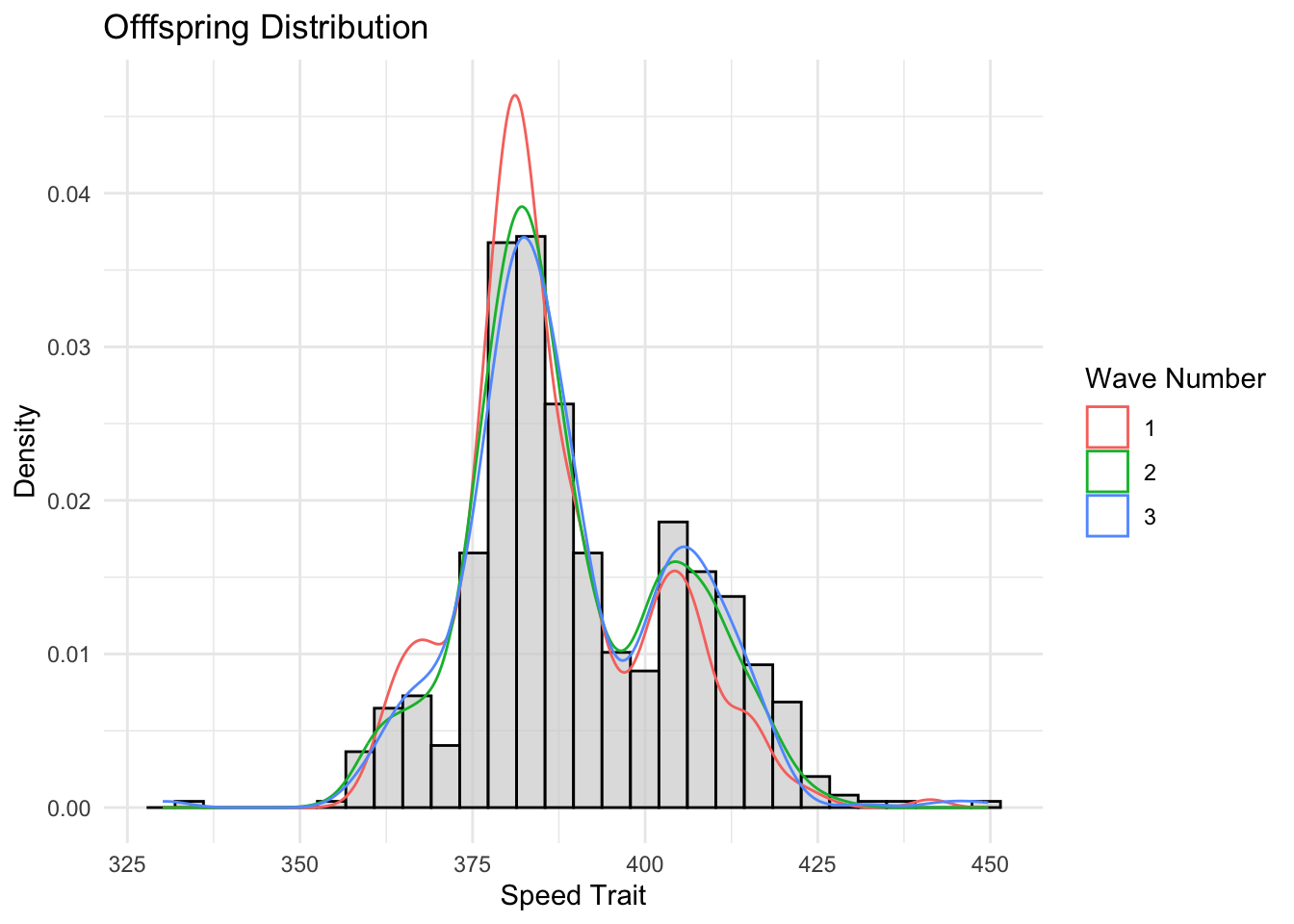
Visualize Basic Trait Patterns
`summarise()` has grouped output by 'file', 'Wave.Number', 'tournament'. You
can override using the `.groups` argument.`geom_smooth()` using method = 'loess' and formula = 'y ~ x'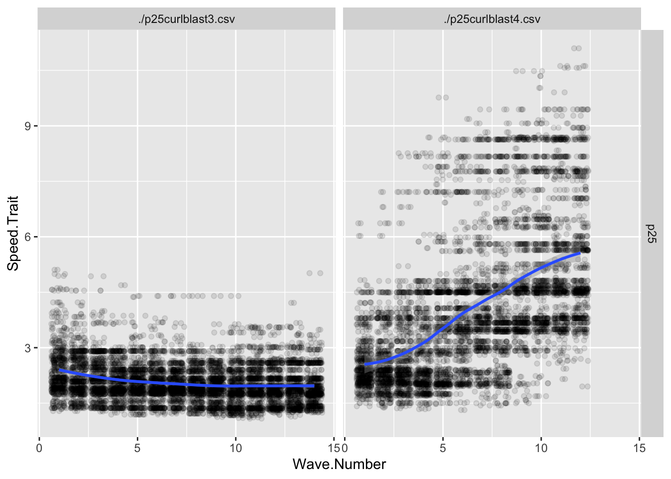
`geom_smooth()` using method = 'loess' and formula = 'y ~ x'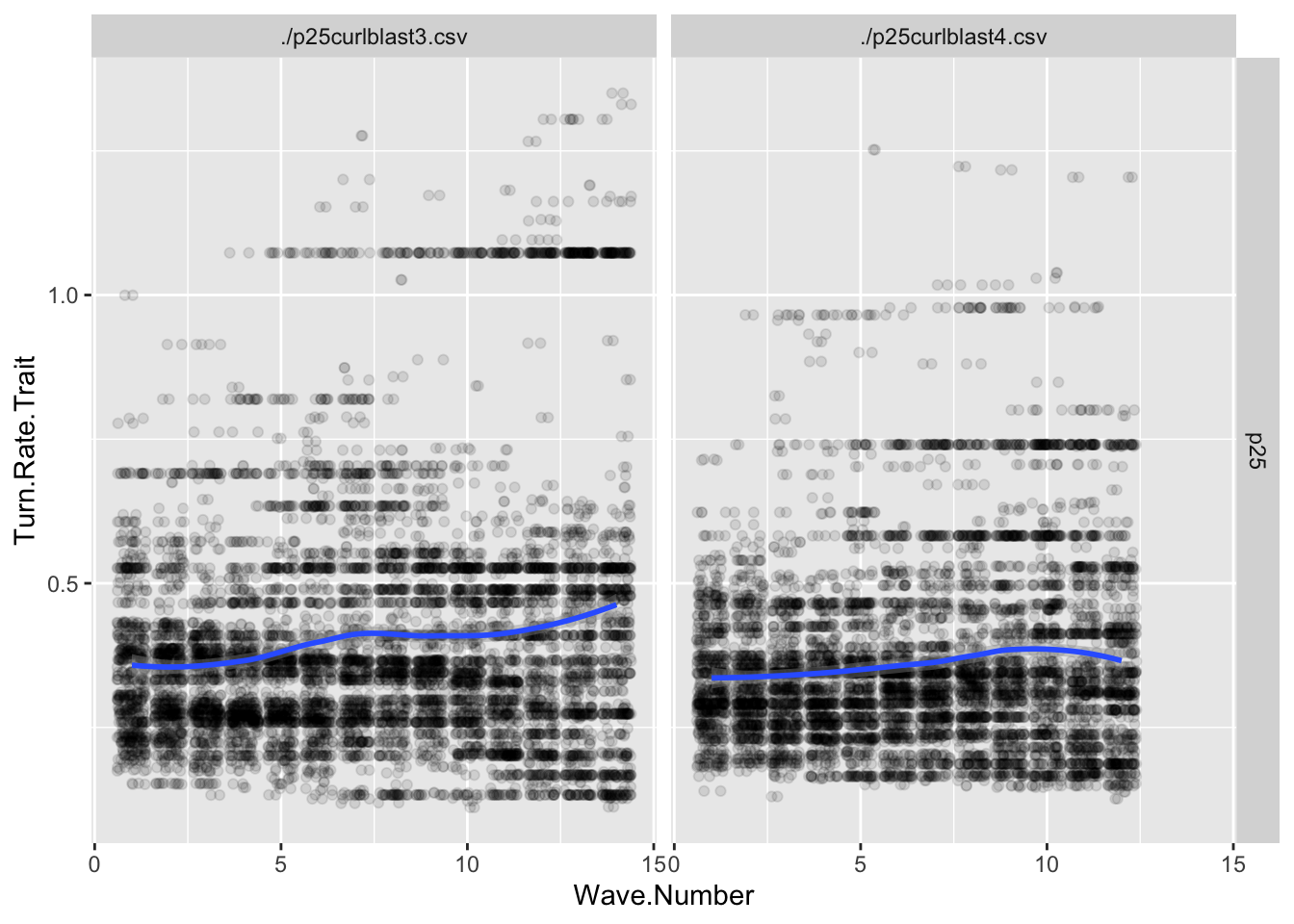
`geom_smooth()` using method = 'loess' and formula = 'y ~ x'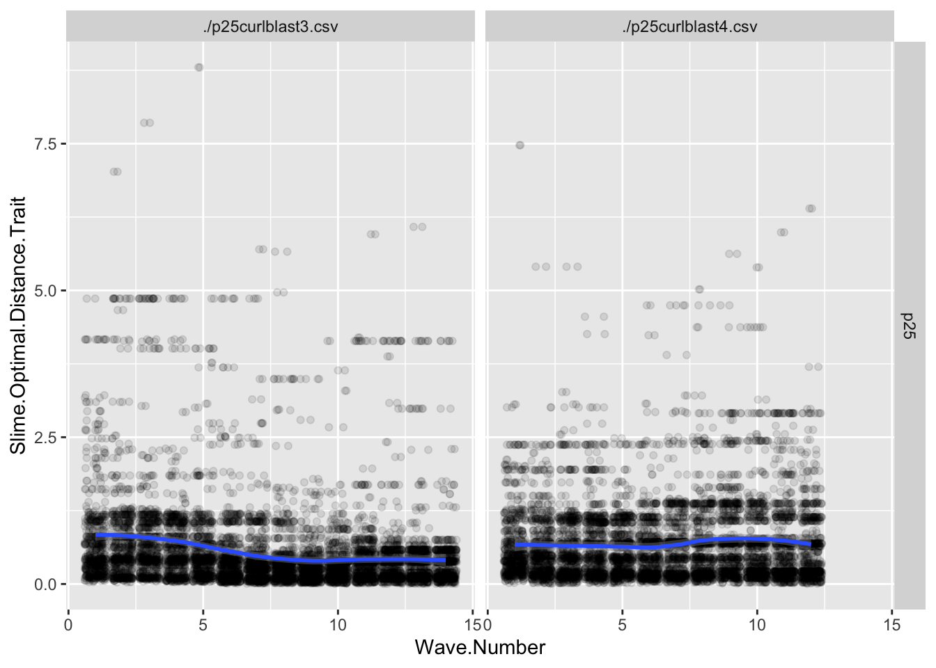
`geom_smooth()` using method = 'loess' and formula = 'y ~ x'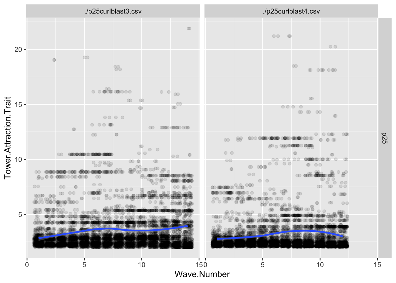
Visualize Basic Type Patterns
`summarise()` has grouped output by 'Wave.Number', 'Main.Type', 'file',
'tournament'. You can override using the `.groups` argument.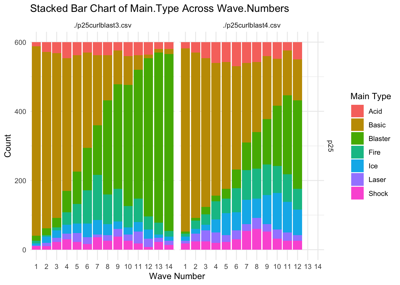
`summarise()` has grouped output by 'Wave.Number', 'Secondary.Type', 'file',
'tournament'. You can override using the `.groups` argument.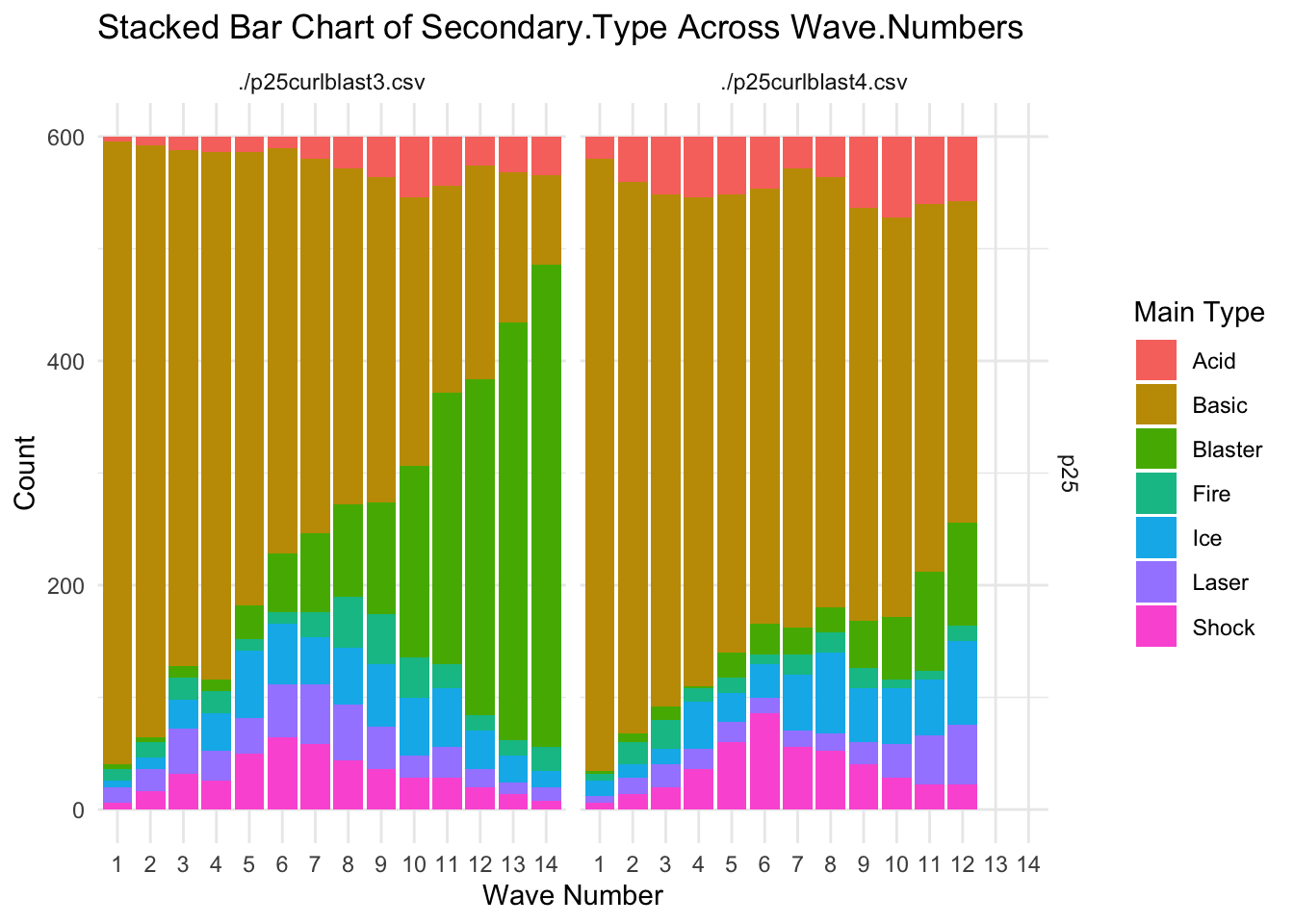
Fitness Analysis
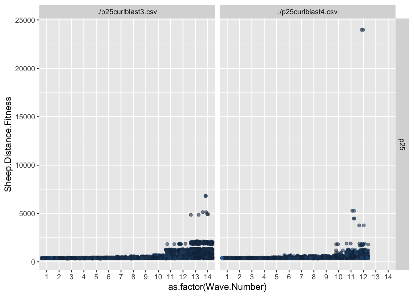
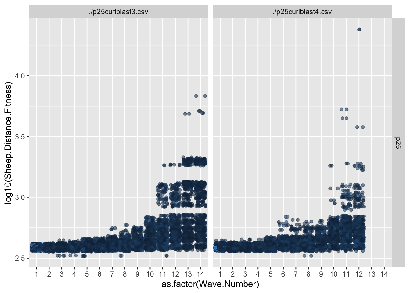
fitness <- ggplot(fit_ranked%>% filter(Wave.Number < max(Wave.Number)), aes(x = Sheep.Distance.Fitness, y = offspring_count))+ geom_point(aes(color = Speed.Trait))+ geom_smooth(method = “lm”)+ facet_grid(Wave.Number~file)
ggsave(fitness, file = “fitness.png”, height = 12, width =4)
fitnessrank <- ggplot(fit_ranked%>% filter(Wave.Number < max(Wave.Number)), aes(x = fitrank, y = offspring_count))+ geom_point(aes(color = Speed.Trait))+ geom_smooth(method = “lm”)+ facet_grid(Wave.Number~file)
ggsave(fitnessrank, file = “fitnessrank.png”, height = 12, width =4)
speed <- ggplot(fit_ranked%>% filter(Wave.Number < max(Wave.Number)), aes(x = Speed.Trait, y = offspring_count))+ geom_point(aes(color = Main.Type))+ geom_smooth(method = “lm”)+ facet_grid(Wave.Number~file)
ggsave(speed, file = “speed.png”, height = 12, width =4)
::: {.cell}
::: {.cell-output .cell-output-stderr}
Warning: The dot-dot notation (..density..) was deprecated in ggplot2 3.4.0. ℹ Please use after_stat(density) instead.
:::

::: {.cell-output .cell-output-stderr}
stat_bin() using bins = 30. Pick better value with binwidth.
:::
::: {.cell-output-display}
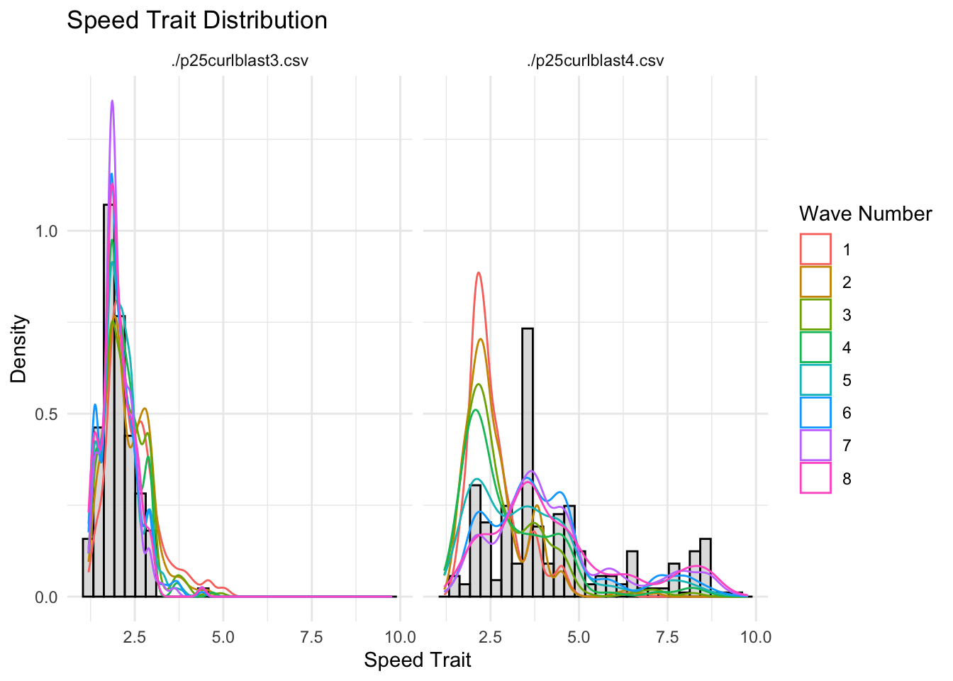{width=672}
:::
::: {.cell-output .cell-output-stderr}
stat_bin() using bins = 30. Pick better value with binwidth.
:::
::: {.cell-output-display}
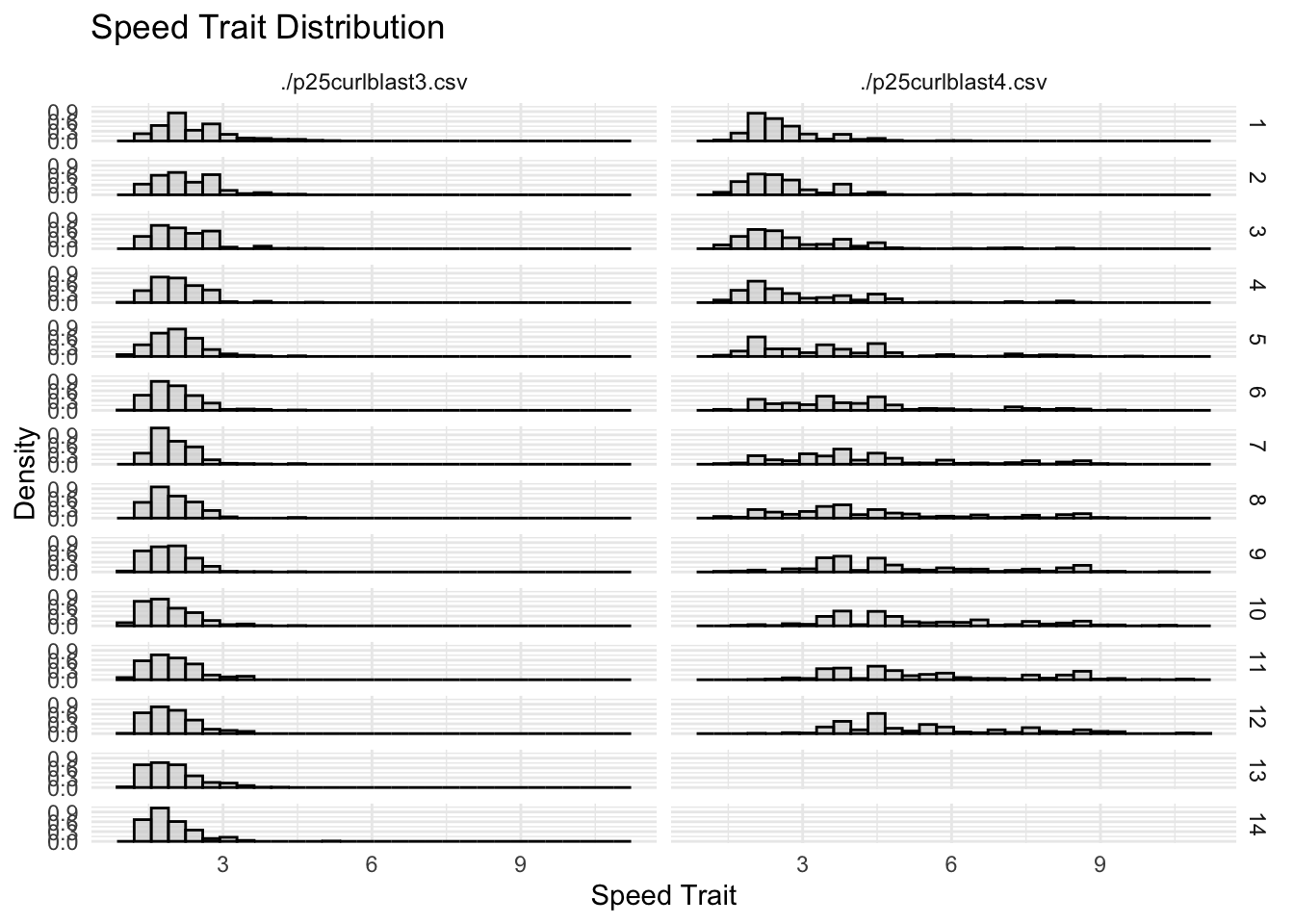{width=672}
:::
::: {.cell-output .cell-output-stderr}
stat_bin() using bins = 30. Pick better value with binwidth. ```
:::
:::
Since this post doesn’t specify an explicit image, the first image in the post will be used in the listing page of posts.